| A simple method to generalize a parametric curve into a
parametric surface is to allow the control points for a curve to vary according
to a set of parametric curves. The following is an example of a Bezier
patch constructed in this fashion.
If we consider a Bezier curve segment, for example, defined by P(s) = S M G_bez, S = [ s^3 s^2 s 1 ], s in [0,1]we can choose to let the elements of G_bez to be Bezier curves: [ P1(t) ] G_bez = [ P2(t) ] [ P3(t) ] [ P4(t) ]where P1(t) = T M G1 P2(t) = T M G2 P3(t) = T M G3 P4(t) = T M G4Each of G1, G2, G3, and G4 are geometry vectors which specify parametric cubic curves in t for one the four control points of the original curve P(s). There are thus 16 values that are needed to specify each of x(s,t), y(s,t) and z(s,t). It would be nice if there was a way to write P(s,t) in a suitably compact way. This can be done as follows. First, transpose the equations for P1(t) ... P4(t) to yield P1(t) = G1^t M^t T^t P2(t) = G2^t M^t T^t P3(t) = G3^t M^t T^t P4(t) = G4^t M^t T^tNow, substitute these equations into our original equation for P(s): P(s) = S M G = S M [ P1(t) ] [ P2(t) ] [ P3(t) ] [ P4(t) ] = S M [ G1^t M^t T^t ] [ G2^t M^t T^t ] [ G3^t M^t T^t ] [ G4^t M^t T^t ] = S M [ g11 g12 g13 g14 ] M^t T^t [ g21 g22 g23 g24 ] [ g31 g32 g33 g34 ] [ g41 g42 g43 g44 ] = S M G_tensor M^t T^tThis is known as a tensor product formulation of a surface. As for the parametric curves, it is really a vector equation, and can thus be written as three separate equations: x(s,t) = S M G_x M^t T^t y(s,t) = S M G_y M^t T^t z(s,t) = S M G_z M^t T^t s,t in [0,1]Each of G_x, G_y, and G_z in the above equations is a 4x4 matrix of scalar values. Bezier Surfaces
Hermite Surfaces (Coon's patch)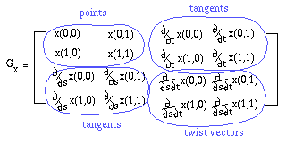 B-spline Surfaces
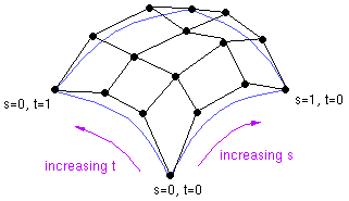
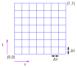
Rendering Bicubic PatchesThe simplest way to convert a bicubic patch into primitives that we already know how to render is to divide it into non-planar quadrilaterals or planar triangles by evaluating P(s,t) at discretized values of s and t, as shown here:
The isoparametric lines in the parameter space thus become isoparametric curves for the final surface. Each of the discretized set of points P(s,t) requires determining [ x(s,t) ] P(s,t) = [ y(s,t) ] [ z(s,t) ]If the evaluations are carried out in a straightforward but inefficient manner, then converting a single patch to quadrilaterals will require 4/(delta_s*delta_t) evaluations of the function P(s,t). We can do better than this, however, if precompute some quantities. It is also possible to make use of the convex hull property for efficient clipping of bezier and b-spline patches. Evaluation Methodsx(s,t) = S M G M^t T^t
precompute S M and store in Q[s] Q[t] = Q^t[s] assuming equal subdivisions in s and t Transformations of Curves and Surfaces
Computing a Surface Normal
N = d/ds P(s,t) x d/dt P(s,t) where |